Using the model wrapper
In the last section we have seen how to run basic samples. Before we get to creating cosmological likelihoods, let us take a look at the model wrapper. It creates a python object that lets you interact with the different parts of your model: theory code, prior and likelihood. It can do the same as the evaluate sampler, and much more, in an interactive way.
You can use it to test your modifications, to evaluate the cosmological observables and likelihoods at particular points, and also to interface cosmological codes and likelihoods with external tools, such as a different sampler, a machine-learning framework…
The basics of model.Model are explained in this short section. We recommend you to take a look at it before going on.
So let us create a simple one using the input generator: Planck 2018 polarized CMB and lensing with CLASS as a theory code. Let us copy the python version (you can also copy the yaml version and load it with yaml_load()).
info_txt = r"""
likelihood:
  planck_2018_lowl.TT:
  planck_2018_lowl.EE:
  planck_NPIPE_highl_CamSpec.TTTEEE: null
  planck_2018_lensing.native: null
theory:
  classy:
    extra_args: {N_ur: 2.0328, N_ncdm: 1}
params:
  logA:
    prior: {min: 2, max: 4}
    ref: {dist: norm, loc: 3.05, scale: 0.001}
    proposal: 0.001
    latex: \log(10^{10} A_\mathrm{s})
    drop: true
  A_s: {value: 'lambda logA: 1e-10*np.exp(logA)', latex: 'A_\mathrm{s}'}
  n_s:
    prior: {min: 0.8, max: 1.2}
    ref: {dist: norm, loc: 0.96, scale: 0.004}
    proposal: 0.002
    latex: n_\mathrm{s}
  H0:
    prior: {min: 40, max: 100}
    ref: {dist: norm, loc: 70, scale: 2}
    proposal: 2
    latex: H_0
  omega_b:
    prior: {min: 0.005, max: 0.1}
    ref: {dist: norm, loc: 0.0221, scale: 0.0001}
    proposal: 0.0001
    latex: \Omega_\mathrm{b} h^2
  omega_cdm:
    prior: {min: 0.001, max: 0.99}
    ref: {dist: norm, loc: 0.12, scale: 0.001}
    proposal: 0.0005
    latex: \Omega_\mathrm{c} h^2
  m_ncdm: {renames: mnu, value: 0.06}
  Omega_Lambda: {latex: \Omega_\Lambda}
  YHe: {latex: 'Y_\mathrm{P}'}
  tau_reio:
    prior: {min: 0.01, max: 0.8}
    ref: {dist: norm, loc: 0.06, scale: 0.01}
    proposal: 0.005
    latex: \tau_\mathrm{reio}
"""

from cobaya.yaml import yaml_load

info = yaml_load(info_txt)

# Add your external packages installation folder
info["packages_path"] = "/path/to/packages"
Now let’s build a model (we will need the path to your external packages’ installation):
from cobaya.model import get_model

model = get_model(info)
To get (log) probabilities and derived parameters for particular parameter values, we can use the different methods of the model.Model (see below), to which we pass a dictionary of sampled parameter values.
Note
Notice that we can only fix sampled parameters: in the example above, the primordial log-amplitude logA is sampled (has a prior) but the amplitude defined from it A_s is not (it just acts as an interface between the sampler and CLASS), so we can not pass it as an argument to the methods of model.Model.
To get a list of the sampled parameters in use:
print(list(model.parameterization.sampled_params()))
Since there are lots of nuisance parameters (most of them coming from planck_2018_highl_plik.TTTEEE), let us be a little lazy and give them random values, which will help us illustrate how to use the model to sample from the prior. To do that, we will use the method sample(), where the class prior.Prior is a member of the Model. If we check out its documentation, we’ll notice that:
It returns an array of samples (hence the
[0]after the call below)Samples are returned as arrays, not a dictionaries, so we need to add the parameter names, whose order corresponds to the output of
model.parameterization.sampled_params().There is an external prior: a gaussian on a linear combination of SZ parameters inherited from the likelihood
planck_2018_highl_plik.TTTEEE; thus, since we don’t know how to sample from it, we need to add theignore_external=Truekeyword (mind that the returned samples are not samples from the full prior, but from the separable 1-dimensional prior described in theparamsblock.
We overwrite our prior sample with some cosmological parameter values of interest, and compute the logposterior (check out the documentation of logposterior() below):
point = dict(
    zip(
        model.parameterization.sampled_params(),
        model.prior.sample(ignore_external=True)[0],
    )
)

point.update(
    {
        "omega_b": 0.0223,
        "omega_cdm": 0.120,
        "H0": 67.01712,
        "logA": 3.06,
        "n_s": 0.966,
        "tau_reio": 0.065,
    }
)

logposterior = model.logposterior(point, as_dict=True)
print("Full log-posterior:")
print("   logposterior:", logposterior["logpost"])
print("   logpriors:", logposterior["logpriors"])
print("   loglikelihoods:", logposterior["loglikes"])
print("   derived params:", logposterior["derived"])
And this will print something like
Full log-posterior:
   logposterior: -16826.4
   logpriors: {'0': -21.068028542859743, 'SZ': -4.4079090809077135}
   loglikelihoods: {'planck_2018_lowl.TT': -11.659342468489626, 'planck_2018_lowl.EE': -199.91123947242667, 'planck_2018_highl_plik.TTTEEE': -16584.946305616675, 'planck_2018_lensing.clik': -4.390708962961917}
   derived params: {'A_s': 2.1327557162026904e-09, 'Omega_Lambda': 0.68165001855872, 'YHe': 0.245273361911158}
Note
0 is the name of the combination of 1-dimensional priors specified in the params block.
Note
Notice that the log-probability methods of Model can take, as well as a dictionary, an array of parameter values in the correct order. This may be useful when using these methods to interact with external codes.
Note
If we try to evaluate the posterior outside the prior bounds, logposterior() will return an empty list for the likelihood values: likelihoods and derived parameters are only computed if the prior is non-null, for the sake of efficiency.
If you would like to evaluate the likelihood for such a point, call loglikes() instead.
Note
If you want to use any of the wrapper log-probability methods with an external code, especially with C or Fortran, consider setting the keyword make_finite=True in those methods, which will return the largest (or smallest) machine-representable floating point numbers, instead of numpy’s infinities.
We can also use the Model to get the cosmological observables that were computed for the likelihood. To see what has been requested from, e.g., the camb theory code, do
print(model.requested())
Which will print something like
{classy: [{'Cl': {'pp': 2048, 'bb': 29, 'ee': 2508, 'tt': 2508, 'eb': 0, 'te': 2508, 'tb': 0}}]}
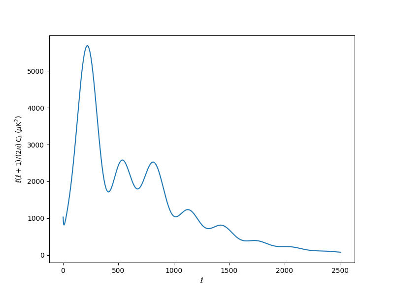
If we take a look at the documentation of must_provide(), we will see that to request the power spectrum we would use the method get_Cl:
Cls = model.provider.get_Cl(ell_factor=True)
import matplotlib.pyplot as plt

plt.figure(figsize=(8, 6))
plt.plot(Cls["ell"][2:], Cls["tt"][2:])
plt.ylabel(r"$\ell(\ell+1)/(2\pi)\,C_\ell\;(\mu \mathrm{K}^2)$")
plt.xlabel(r"$\ell$")
plt.savefig("cltt.png")
# plt.show()
Warning
Cosmological observables requested this way always correspond to the last set of parameters with which the likelihood was evaluated.
If we want to request additional observables not already requested by the likelihoods, we can use the method must_provide() of the theory code (check out its documentation for the syntax).
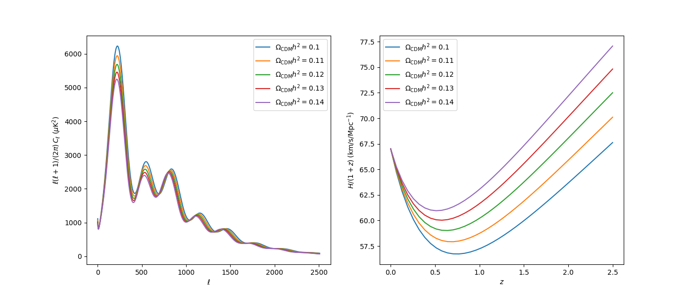
As a final example, let us request the Hubble parameter for a number of redshifts and plot both it and the power spectrum for a range of values of \(\Omega_\mathrm{CDM}h^2\):
# Request H(z)
import numpy as np

redshifts = np.linspace(0, 2.5, 40)
model.add_requirements({"Hubble": {"z": redshifts}})

omega_cdm = [0.10, 0.11, 0.12, 0.13, 0.14]

f, (ax_cl, ax_h) = plt.subplots(1, 2, figsize=(14, 6))
for o in omega_cdm:
    point["omega_cdm"] = o
    model.logposterior(point)  # to force computation of theory
    Cls = model.provider.get_Cl(ell_factor=True)
    ax_cl.plot(Cls["ell"][2:], Cls["tt"][2:], label=r"$\Omega_\mathrm{CDM}h^2=%g$" % o)
    H = model.provider.get_Hubble(redshifts)
    ax_h.plot(redshifts, H / (1 + redshifts), label=r"$\Omega_\mathrm{CDM}h^2=%g$" % o)
ax_cl.set_ylabel(r"$\ell(\ell+1)/(2\pi)\,C_\ell\;(\mu \mathrm{K}^2)$")
ax_cl.set_xlabel(r"$\ell$")
ax_cl.legend()
ax_h.set_ylabel(r"$H/(1+z)\;(\mathrm{km}/\mathrm{s}/\mathrm{Mpc}^{-1})$")
ax_h.set_xlabel(r"$z$")
ax_h.legend()
plt.savefig("omegacdm.png")
# plt.show()
If you are creating several models in a single session, call close() after you are finished with each one, to release the memory it has used.
If you had set timing=True in the input info, dump_timing() would print the average computation time of your likelihoods and theory code (see the bottom of section Creating your own cosmological likelihood for a use example).
Note
If you are not really interested in any likelihood value and just want to get some cosmological observables (possibly using your modified version of a cosmological code), use the mock ‘one’ likelihood as the only likelihood, and add the requests for cosmological quantities by hand, as we did above with \(H(z)\).
NB: you will not be able to request some of the derived parameters unless you have requested some cosmological product to compute.
Warning
Unfortunately, not all likelihoods and cosmological codes are instance-safe, e.g. you can’t define two models using each the unbinned TT and TTTEEE likelihoods at the same time.
To sample from your newly-create model’s posterior, it is preferable to pass it directly to a sampler, as opposed to calling run(), which would create yet another instance of the same model, taking additional time and memory. To do that, check out this section.
Low-level access to the theory code
Besides the results listed in must_provide(), you may be able to access other cosmological quantities from the Boltzmann code, see Access to CAMB computation products and Access to CLASS computation products.