Advanced example

In this example, we will see how to sample from priors and likelihoods given as Python functions, and how to dynamically define new parameters. This time, we will start from the interpreter and then learn how to create a pure yaml input file with the same information.

Note

You can play with an interactive version of this example here.

From a Python interpreter

Our likelihood will be a gaussian quarter ring centred at 0, with radius 1. We define it with the following Python function

import numpy as np
from scipy import stats


def gauss_ring_logp(x, y, mean_radius=1, std=0.02):
    """
    Defines a gaussian ring likelihood on cartesian coordinater,
    around some ``mean_radius`` and with some ``std``.
    """
    return stats.norm.logpdf(np.sqrt(x**2 + y**2), loc=mean_radius, scale=std)

Note

NB: external likelihood and priors (as well as internal ones) must return log-probabilities.

And we add it to the information dictionary like this:

info = {"likelihood": {"ring": gauss_ring_logp}}

cobaya will automatically recognise x and y (or whatever parameter names of your choice) as the input parameters of that likelihood, which we have named ring. Let’s define a prior for them:

info["params"] = {
    "x": {"prior": {"min": 0, "max": 2}, "ref": 0.5, "proposal": 0.01},
    "y": {"prior": {"min": 0, "max": 2}, "ref": 0.5, "proposal": 0.01}}

Now, let’s assume that we want to track the radius of the ring, whose posterior will be approximately gaussian, and the angle over the \(x\) axis, whose posterior will be uniform. We can define them as functions of known input parameters:

def get_r(x, y):
    return np.sqrt(x ** 2 + y ** 2)


def get_theta(x, y):
    return np.arctan(y / x)

info["params"]["r"] = {"derived": get_r}
info["params"]["theta"] = {"derived": get_theta,
                           "latex": r"\theta", "min": 0, "max": np.pi/2}

Note

The options min and max for theta do not define a prior (theta is not a sampled parameter!), but the range used by GetDist for the derived theta when calculating kernel density estimates and plotting the marginal distributions.

Now, we add the sampler information and run. Notice the high number of samples requested for just two dimensions, in order to map the curving posterior accurately, and the large limit on tries before chain gets stuck:

info["sampler"] = {"mcmc": {"Rminus1_stop": 0.001, "max_tries": 1000}}

from cobaya import run
updated_info, sampler = run(info)

Here Rminus1_stop is the tolerance for deciding when the chains are converged, with a smaller number meaning better convergence (defined as R-1, diagonalized Gelman-Rubin parameter value at which chains should stop).

Note

If using MPI and the MCMC sampler, take a look at this section.

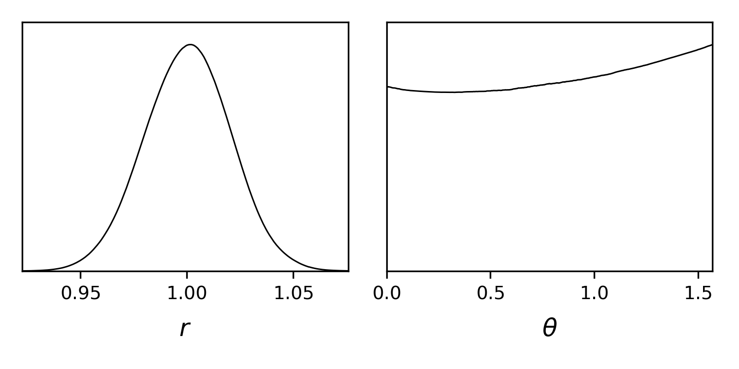
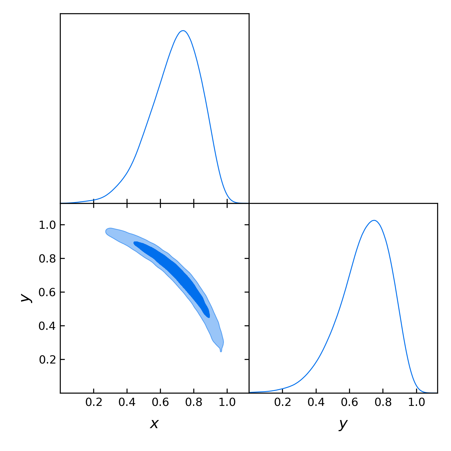
Let us plot the posterior for x, y, the radius and the angle:

%matplotlib inline
import getdist.plots as gdplt

gdsamples = sampler.products(to_getdist=True)["sample"]
gdplot = gdplt.get_subplot_plotter(width_inch=5)
gdplot.triangle_plot(gdsamples, ["x", "y"], filled=True)
gdplot = gdplt.get_subplot_plotter(width_inch=5)
gdplot.plots_1d(gdsamples, ["r", "theta"], nx=2)

Now let’s assume that we are only interested in some region along x=y, defined by a gaussian perpendicular to that direction. We can add this constraint as an external prior, in a similar way the external likelihood was added. The logprior for this can be added simply as:

info["prior"] = {"x_eq_y_band":
                 lambda x, y: stats.norm.logpdf(x - y, loc=0, scale=0.3)}

Let’s run with the same configuration and analyse the output:

updated_info_x_eq_y, sampler_x_eq_y = run(info)

gdsamples_x_eq_y = MCSamplesFromCobaya(
    updated_info_x_eq_y, sampler_x_eq_y.products()["sample"])
gdplot = gdplt.get_subplot_plotter(width_inch=5)
gdplot.triangle_plot(gdsamples_x_eq_y, ["x", "y"], filled=True)

Alternative: `r` and `theta` defined inside the likelihood function

Custom likelihoods also allow for the definition of derived parameters. In this example, it would make sense for r and theta to be computed inside the likelihood. To do that, we would redefine the likelihood as follows (see details at External likelihood functions):

# List available derived parameters in the 'output_params' option of the likelihood.
# To make room for that, you need assign the function to the option 'external'.
# Return both the log-likelihood and a dictionary of derived parameters.
def gauss_ring_logp_with_derived(x, y):
    r = np.sqrt(x**2+y**2)
    derived = {"r": r, "theta": np.arctan(y/x)}
    return stats.norm.logpdf(r, loc=1, scale=0.02), derived

info_alt = {"likelihood": {"ring":
    {"external": gauss_ring_logp_with_derived, "output_params": ["r", "theta"]}}}

And remove the definition (but not the mention!) of r and theta in the params block:

info_alt["params"] = {
    "x": {"prior": {"min": 0, "max": 2}, "ref": 0.5, "proposal": 0.01},
    "y": {"prior": {"min": 0, "max": 2}, "ref": 0.5, "proposal": 0.01},
    "r": None,
    "theta": {"latex": r"\theta", "min": 0, "max": np.pi/2}}

info_alt["prior"] = {"x_eq_y_band":
                  lambda x, y: stats.norm.logpdf(x - y, loc=0, scale=0.3)}

Even better: sampling directly on `r` and `theta`

r and theta are better variables with which to sample this posterior: the gaussian ring is an approximate gaussian on r (and uniform on theta), and the x = y band is an approximate gaussian on theta. Given how much simpler the posterior is in these variables, we should expect a more accurate result with the same number of samples, since now we don’t have the complication of having to go around the ring.

Of course, in principle we would modify the likelihood to take r and theta instead of x and y. But let us assume that this is not easy or even not possible.

Our goal can still be achieved in a simple way at the parameterization level only, i.e. without needing to modify the parameters that the likelihood takes, as explained in Defining parameters dynamically. In essence:

We give a prior to the parameters over which we want to sample, here r and theta, and signal that they are not to passed to the likelihood by giving them the property drop: True.
We define the parameters taken by the likelihood, here x and y, as functions of the parameters we want to sample over, here r and theta. By default, their values will be saved to the chain files.

Starting from the info of the original example (not the one with theta and r as derived parameters of the likelihood):

from copy import deepcopy
info_rtheta = deepcopy(info)
info_rtheta["params"] = {
    "r": {"prior": {"min": 0, "max": 2}, "ref": 1,
          "proposal": 0.01, "drop": True},
    "theta": {"prior": {"min": 0, "max": np.pi/2}, "ref": 0,
               "proposal": 0.5, "latex": r"\theta", "drop": True},
    "x": {"value" : lambda r,theta: r*np.cos(theta), "min": 0, "max": 2},
    "y": {"value" : lambda r,theta: r*np.sin(theta), "min": 0, "max": 2}}

# The priors above are just linear with specific ranges. There is also a Jacobian
# from the change of variables, which we can include as an additional prior.
# Here the Jacobian is just proportional to r (log-prior is proportional to log(r))
info_rtheta["prior"] = {"Jacobian" : lambda r: np.log(r)}

To also sample with the band prior, we’d reformulate it in terms of the new parameters

info_rtheta["prior"]["x_eq_y_band"] = lambda r, theta: stats.norm.logpdf(
    r * (np.cos(theta) - np.sin(theta)), loc=0, scale=0.3)

From the shell

To run the example above in from the shell, we could just save all the Python code above in a .py file and run it with python [file_name]. To get the sampling results as text output, we would add to the info dictionary some output prefix, e.g. info["output"] = "chains/ring".

But there a small complication: cobaya would fail at the time of dumping a copy of the information dictionary, since there is no way to dump a pure Python function to pure-text yaml in a reproducible manner. To solve that, for functions that can be written in a single line, we simply write it lambda form and wrap it in quotation marks, e.g. for r that would be "lambda x,y: np.sqrt(x**2+y**2)". Inside these lambdas, you can use np for numpy and stats for scipy.stats.

More complex functions must be saved into a separate file and imported on the fly. In the example above, let’s assume that we have saved the definition of the gaussian ring likelihood (which could actually be written in a single line anyway), to a file called my_likelihood in the same folder as the Python script. In that case, we should be able to load the likelihood as

# Notice the use of single vs double quotes
info = {"likelihood": {"ring": "import_module('my_likelihood').gauss_ring_logp"}}

With those changes, we would be able to run our Python script from the shell (with MPI, if desired) and have the chains saved where requested.

Bu we could also have incorporated those text definitions into a yaml file, that we could call with cobaya-run:

likelihood:
  ring: import_module('my_likelihood').gauss_ring_logp

params:
  x:
    prior: {min: 0, max: 2}
    ref: 0.5
    proposal: 0.01
  y:
    prior: {min: 0, max: 2}
    ref: 0.5
    proposal: 0.01
  r:
    derived: 'lambda x,y: np.sqrt(x**2+y**2)'
  theta:
    derived: 'lambda x,y: np.arctan(y/x)'
    latex: \theta
    min: 0
    max: 1.571  # =~ pi/2

prior:
  x_eq_y_band: 'lambda x,y: stats.norm.logpdf(
                   x - y, loc=0, scale=0.3)'

sampler:
  mcmc:
    Rminus1_stop: 0.001

output: chains/ring

Note

Notice that we need the quotes around the definition of the lambda functions, or yaml would get confused by the :.

If we would like to sample on theta and r instead, our input file would be:

likelihood:
  ring: import_module('my_likelihood').gauss_ring_logp

params:
  r:
    prior: {min: 0, max: 2}
    ref: 1
    proposal: 0.01
    drop: True
  theta:
    prior: {min: 0, max: 1.571}  # =~ [0, pi/2]
    ref: 0
    proposal: 0.5
    latex: \theta
    drop: True
  x:
    value: 'lambda r,theta: r*np.cos(theta)'
    min: 0
    max: 2
  y:
    value: 'lambda r,theta: r*np.sin(theta)'
    min: 0
    max: 2

prior:
  Jacobian: 'lambda r: np.log(r)'
  x_eq_y_band: 'lambda r, theta: stats.norm.logpdf(
      r * (np.cos(theta) - np.sin(theta)), loc=0, scale=0.3)'

sampler:
  mcmc:
    Rminus1_stop: 0.001

output: chains/ring

Advanced example

From a Python interpreter

Alternative: r and theta defined inside the likelihood function

Even better: sampling directly on r and theta

From the shell

Alternative: `r` and `theta` defined inside the likelihood function

Even better: sampling directly on `r` and `theta`