Quickstart example
Let us present here a simple example, without explaining much about it — each of its aspects will be broken down in the following sections.
We will run it first from the shell, and later from a Python interpreter (or a Jupyter notebook).
From the shell
The input of cobaya consists of a text file that usually looks like this:
likelihood:
  gaussian_mixture:
    means: [0.2, 0]
    covs: [[0.1, 0.05], [0.05,0.2]]
    derived: True

params:
  a:
    prior:
      min: -0.5
      max: 3
    latex: \alpha
  b:
    prior:
      dist: norm
      loc: 0
      scale: 1
    ref: 0
    proposal: 0.5
    latex: \beta
  derived_a:
    latex: \alpha^\prime
  derived_b:
    latex: \beta^\prime

sampler:
  mcmc:

output: chains/gaussian
You can see the following blocks up there:
A
likelihoodblock, listing the likelihood pdf’s to be explored, here a gaussian with the mean and covariance stated.A
paramsblock, stating the parameters that are going to be explored (or derived), theirprior, the the Latex label that will be used in the plots, the reference (ref) starting point for the chains (optional), and the initial spread of the MCMC covariance matrixproposal.A
samplerblock stating that we will use themcmcsampler to explore the prior+likelihood described above, stating the maximum number of samples used, how many initial samples to ignore, and that we will sequentially refine our initial guess for a covariance matrix.An
outputprefix, indicating where the products will be written and a prefix for their name.
To run this example, save the text above in a file called gaussian.yaml in a folder of your choice, and do
$ cobaya-run gaussian.yaml
or alternatively (if shell scripts are not available or ambiguously defined):
$ python -m cobaya gaussian.yaml
Note
Cobaya is MPI-aware. If you have installed mpi4py (see this section), you can run
$ mpirun -n [n_processes] cobaya-run gaussian.yaml
which will converge faster!
After a few seconds, a folder named chains will be created, and inside it you will find three files:
chains
├── gaussian.input.yaml
├── gaussian.updated.yaml
└── gaussian.1.txt
The first file reproduces the same information as the input file given, here gaussian.yaml. The second contains the updated information needed to reproduce the sample, similar to the input one, but populated with the default options for the sampler, likelihood, etc. that you have used.
The third file, ending in .txt, contains the MCMC sample, and its first lines should look like
# weight  minuslogpost         a         b  derived_a  derived_b  minuslogprior  minuslogprior__0      chi2  chi2__gaussian
    10.0      4.232834  0.705346 -0.314669   1.598046  -1.356208       2.221210          2.221210  4.023248        4.023248
     2.0      4.829217 -0.121871  0.693151  -1.017847   2.041657       2.411930          2.411930  4.834574        4.834574
You can run a posterior maximization process on top of the Monte Carlo sample (using its maximum as starting point) by repeating the shell command with a --minimize flag:
$ cobaya-run gaussian.yaml --minimize
You can use GetDist to analyse the results of this sample: get marginalized statistics, convergence diagnostics and some plots. We recommend using the graphical user interface. Simply run getdist-gui from anywhere, press the green + button, navigate in the pop-up window into the folder containing the chains (here chains) and click choose. Now you can get some result statistics from the Data menu, or generate some plots like this one (just mark the the options in the red boxes and hit Make plot):
Note
You can add an option label: non-latex $latex$ to your info, and it will be used as legend label when plotting multiple samples.
Note
The default mcmc method uses automated proposal matrix learning. You may need to discard the first section of the chain as burn in.
In getdist-gui see analysis settings on the Option menu, and change ignore_rows to, e.g., 0.3 to discard the first 30% of each chain.
Note
For a detailed user manual and many more examples, check out the GetDist documentation!
From a Python interpreter
You can use cobaya interactively within a Python interpreter or a Jupyter notebook. This will allow you to create input and process products programatically, making it easier to streamline a complicated analyses.
The actual input information of cobaya is provided as Python dictionaries (a yaml file is just a representation of a dictionary). We can easily define the same information above as a dictionary:
info = {
    "likelihood": {
        "gaussian_mixture": {
            "means": [0.2, 0],
            "covs": [[0.1, 0.05], [0.05, 0.2]],
            "derived": True,
        }
    },
    "params": dict(
        [
            ("a", {"prior": {"min": -0.5, "max": 3}, "latex": r"\alpha"}),
            (
                "b",
                {
                    "prior": {"dist": "norm", "loc": 0, "scale": 1},
                    "ref": 0,
                    "proposal": 0.5,
                    "latex": r"\beta",
                },
            ),
            ("derived_a", {"latex": r"\alpha^\prime"}),
            ("derived_b", {"latex": r"\beta^\prime"}),
        ]
    ),
    "sampler": {"mcmc": None},
}
The code above may look more complicated than the corresponding yaml one, but in exchange it is much more flexible, allowing you to quick modify and swap different parts of it.
Notice that here we suppress the creation of the chain files by not including the field output, since this is a very basic example. The chains will therefore only be loaded in memory.
Note
Add this snippet after defining your info to be able to use the cobaya-run arguments -d (debug), -f (force) and -r (resume) when launching your Python script from the shell:
import sys
for k, v in {"-f": "force", "-r": "resume", "-d": "debug"}.items():
    if k in sys.argv:
        info[v] = True
Alternatively, we can load the input from a yaml file like the one above:
from cobaya.yaml import yaml_load_file

info_from_yaml = yaml_load_file("gaussian.yaml")
And info, info_from_yaml and the file gaussian.yaml should contain the same information (except that we have chosen not to add an output prefix to info).
Now, let’s run the example.
from cobaya.run import run

updated_info, sampler = run(info)
Note
If using MPI and the MCMC sampler, take a look at this section.
The run function returns two variables:
An information dictionary updated with the defaults, equivalent to the
updatedyaml file produced by the shell invocation.A sampler object, with a
sampler.products()being a dictionary of results. For themcmcsampler, the dictionary contains only one chain under the keysample.
Note
To run a posterior maximization process after the Monte Carlo run, the simplest way is to repeat the run call with a minimize=True flag, saving the return values with a different name:
updated_info_minimizer, minimizer = run(info, minimize=True)
# To get the maximum-a-posteriori:
print(minimizer.products()["minimum"])
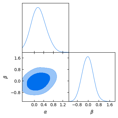
Let’s now analyse the chain and get some plots, using the interactive interface to GetDist instead of the GUI used above:
# Export the results to GetDist
gd_sample = sampler.products(to_getdist=True)["sample"]

# Analyze and plot
mean = gd_sample.getMeans()[:2]
covmat = gd_sample.getCovMat().matrix[:2, :2]
print("Mean:")
print(mean)
print("Covariance matrix:")
print(covmat)
# %matplotlib inline  # uncomment if running from the Jupyter notebook
import getdist.plots as gdplt

gdplot = gdplt.get_subplot_plotter()
gdplot.triangle_plot(gd_sample, ["a", "b"], filled=True)
Output:
Mean:
[ 0.19495375 -0.02323249]
Covariance matrix:
[[ 0.0907666   0.0332858 ]
 [ 0.0332858   0.16461655]]
Alternatively, if we had chosen to write the output as in the shell case by adding an output prefix, we could have loaded the chain in GetDist format from the hard drive:
# Export the results to GetDist
from cobaya import load_samples

gd_sample = load_samples(info["output"], to_getdist=True)

# Analyze and plot
# [Exactly the same here...]
If we are only interested in plotting, we do not even need to generate a GetDist MCSamples object: we can ask the plotter to load all chains in the given folder, and then just name the corresponding one when plotting:
# Just plotting (loading on-the-fly)
# Notice that GetDist requires a full path when loading samples
import os

import getdist.plots as gdplt

folder, name = os.path.split(os.path.abspath(info["output"]))
gdplot = gdplt.get_subplot_plotter(chain_dir=folder)
gdplot.triangle_plot(name, ["a", "b"], filled=True)