mcmc sampler
Note
If you use this sampler, please cite it as:
A. Lewis and S. Bridle, “Cosmological parameters from CMB and other data: A Monte Carlo approach”
(arXiv:astro-ph/0205436)
A. Lewis, “Efficient sampling of fast and slow cosmological parameters”
(arXiv:1304.4473)
If you use fast-dragging, you should also cite
R.M. Neal, “Taking Bigger Metropolis Steps by Dragging Fast Variables”
(arXiv:math/0502099)
This is the Markov Chain Monte Carlo Metropolis sampler used by CosmoMC, and described in Lewis, “Efficient sampling of fast and slow cosmological parameters” (arXiv:1304.4473). It works well on simple uni-modal (or only weakly multi-modal) distributions.
The proposal pdf is a gaussian mixed with an exponential pdf in random directions, which is more robust to misestimation of the width of the proposal than a pure gaussian. The scale width of the proposal can be specified per parameter with the property proposal (it defaults to the standard deviation of the reference pdf, if defined, or the prior’s one, if not). However, initial performance will be much better if you provide a covariance matrix, which overrides the default proposal scale width set for each parameter.
Note
The proposal width for a parameter should be close to its conditional posterior, not its marginalized width. For strong degeneracies the latter can be much wider than the former, and hence it could cause the chain to get stuck.
Underestimating a good proposal width is usually better than overestimating it: an underestimate can be rapidly corrected by the adaptive covariance learning, but if the proposal width is too large the chain may never move at all.
If the distribution being sampled is known have tight strongly non-linear parameter degeneracies, re-define the sampled parameters to remove the degeneracy before sampling (linear degeneracies are not a problem, esp. if you provide an approximate initial covariance matrix).
Initial point for the chains
The initial points for the chains are sampled from the reference pdf (see Parameters and priors). If the reference pdf is a fixed point, chains will always start from that point. If there is no reference pdf defined for a parameter, the initial sample is drawn from the prior instead.
Example of parameters block:
params:
  a:
   prior:
     min: -2
     max:  2
   ref:
     min: -1
     max:  1
   proposal: 0.5
   latex: \alpha

  b:
   prior:
     min: -1
     max:  4
   ref: 2
   proposal: 0.25
   latex: \beta
  c:
   prior:
     min: -1
     max:  1
   ref:
     dist: norm
     loc: 0
     scale: 0.2
   latex: \gamma
a– the initial point of the chain is drawn from an uniform pdf between -1 and 1.b– the initial point of the chain is always atb=2.c– the initial point of the chain is drawn from a gaussian centred at 0 with standard deviation 0.2.
Fixing the initial point is not usually recommended, since to assess convergence it is useful to run multiple chains (which you can do in parallel using MPI), and use the difference between the chains to assess convergence: if the chains all start in exactly the same point, they could appear to have converged just because they started at the same place. On the other hand if your initial points are spread much more widely than the posterior it could take longer for chains to converge.
Covariance matrix of the proposal pdf
An accurate, or even approximate guess for the proposal pdf will normally lead to significantly faster convergence.
In Cobaya, the covariance matrix of the proposal pdf is optionally indicated through mcmc’s property covmat, either as a file name (including path, absolute or relative to the invocation folder), or as an actual matrix. If a file name is given, the first line of the covmat file must start with #, followed by a list of parameter names, separated by a space. The rest of the file must contain the covariance matrix,
one row per line.
An example for the case above:
# a     b
  0.1   0.01
  0.01  0.2
Instead, if given as a matrix, you must also include the covmat_params property, listing the parameters in the matrix in the order in which they appear. Finally, covmat admits the special value auto that searches for an appropriate covariance matrix in a database (see Basic cosmology runs).
If you do not know anything about the parameters’ correlations in the posterior, instead of specifying the covariance matrix via MCMC’s covmat field, you may simply add a proposal field to the sampled parameters, containing the expected standard deviation of the proposal. In the absence of a parameter in the covmat which also lacks its own proposal property, the standard deviation of the reference pdf (of prior if not given) will be used instead (though you would normally like to avoid that possibility by providing at least a proposal property, since guessing it from the prior usually leads to a very small initial acceptance rate, and will tend to get your chains stuck).
Note
A covariance matrix given via covmat does not need to contain the all the sampled parameters, and may contain additional ones unused in your run. For the missing parameters the specified input proposal (or reference, or prior) is used, assuming no correlations.
If the covariance matrix shown above is used for the previous example, the final covariance matrix of the proposal will be:
# a     b     c
  0.1   0.01  0
  0.01  0.2   0
  0     0     0.04
If the option learn_proposal is set to True, the covariance matrix will be updated regularly. This means that a high accuracy of the initial covariance is not critical (just make sure your proposal widths are sufficiently small that chains can move and hence explore the local shape; if your widths are too wide the parameter may just get stuck).
If you are not sure that your posterior has one single mode, or if its shape is very irregular, you may want to set learn_proposal: False; however the MCMC sampler is not likely to work well in this case and other samplers designed for multi-modal distributions (e.g. PolyChord) may be a better choice.
If you do not know how good your initial guess for the starting point and covariance is, a number of initial burn in samples can be ignored from the start of the chains (e.g. 10 per dimension). This can be specified with the parameter burn_in. These samples will be ignored for all purposes (output, convergence, proposal learning…). Of course there may well also be more burn in after these points are discarded, as the chain points converge (and, using learn_proposal, the proposal estimates also converge). Often removing the first 30% the entire final chains gives good results (using ignore_rows=0.3 when analysing with getdist).
Taking advantage of a speed hierarchy
In Cobaya, the proposal pdf is blocked by speeds, i.e. it allows for efficient sampling of a mixture of fast and slow parameters, such that we can avoid recomputing the slowest parts of the likelihood calculation when sampling along the fast directions only. This is often very useful when the likelihoods have large numbers of nuisance parameters, but recomputing the likelihood for different sets of nuisance parameters is fast.
Two different sampling schemes are available in the mcmc sampler to take additional advantage of a speed hierarchy:
Oversampling the fast parameters: consists simply of taking more steps in the faster directions, useful when exploring their conditional distributions is cheap. Enable it by setting
oversample_powerto any value larger than 0 (1 means spending the same amount of time in all parameter blocks; you will rarely want to go over that value).Dragging the fast parameters: consists of taking a number of intermediate fast steps when jumping between positions in the slow parameter space, such that (for large numbers of dragging steps) the fast parameters are dragged along the direction of any degeneracy with the slow parameters. Enable it by setting
drag: True. You can control the relative amount of fast vs slow samples with the sameoversample_powerparameter.
In general, the dragging method is the recommended one if there are non-trivial degeneracies between fast and slow parameters that are not well captured by a covariance matrix, and you have a fairly large speed hierarchy. Oversampling can potentially produce very large output files (less so if the oversample_thin option is left to its default True value); dragging outputs smaller chain files since fast parameters are effectively partially marginalized over internally. For a thorough description of both methods and references, see A. Lewis, “Efficient sampling of fast and slow cosmological parameters” (arXiv:1304.4473).
The relative speeds can be specified per likelihood/theory, with the option speed, preferably in evaluations per second (approximately). The speeds can also be measured automatically when you run a chain (with mcmc, measure_speeds: True), allowing for variations with the number of threads used and machine differences. This option only tests the speed on one point (per MPI instance) by default, so if your speed varies significantly with where you are in parameter space it may be better to either turn the automatic selection off and keep to manually specified average speeds, or to pass a large number instead of True as the value of measure_speeds (it will evaluate the posterior that many times, so the chains will take longer to initialise).
To manually measure the average speeds, set measure_speeds in the mcmc block to a high value and run your input file with the --test option; alternatively, add timing: True at the highest level of your input (i.e. not inside any of the blocks), set the mcmc options burn_in: 0 and max_samples to a reasonably large number (so that it will be done in a few minutes), and check the output: it should have printed, towards the end, computation times for the likelihood and theory codes in seconds, the inverse of which are the speeds.
If the speed has not been specified for a component, it is assigned the slowest one in the set. If two or more components with different speeds share a parameter, said parameter is assigned to a separate block with a speed that takes into account the computation time of all the codes that depends on it.
For example:
theory:
  theory_code:
    speed: 2

likelihood:
  like_a:
  like_b:
    speed: 4
Here, evaluating the theory code is the slowest step, while the like_b is faster. Likelihood like_a is assumed to be as slow as the theory code.
Manual specification of speed blocking
Automatic speed blocking takes advantage of differences in speed per likelihood (or theory). If the parameters of your likelihood or theory have some internal speed hierarchy that you would like to exploit (e.g. if your likelihood internally caches the result of a computation depending only on a subset of the likelihood parameters), you can specify a fine-grained list of parameter blocks and their oversampling factors, using the mcmc option blocking.
E.g. if a likelihood depends of parameters a, b and c and the cost of varying a is twice as big as the other two, your mcmc block should look like
mcmc:
  blocking:
    - [1, [a]]
    - [2, [b,c]]
  # drag: True  # if desired; 2 different oversampling factors only!
Warning
When choosing an oversampling factor, one should take into account the total cost of varying one parameter in the block, i.e. the time needed to re-compute every part of the code that depends (directly or indirectly) on it.
For example, if varying parameter a in the example above would also force a re-computation of the part of the code associated to parameters b and c, then the relative cost of varying the parameters in each block would not be 2-to-1, but (2+1)-to-1, meaning oversampling factors of 1 and 3 may be more appropriate.
Note
If blocking is specified, it must contain all the sampled parameters.
Note
If automatic learning of the proposal covariance is enabled, after some checkpoint the proposed steps will mix parameters from different blocks, but always towards faster ones. Thus, it is important to specify your blocking in ascending order of speed, when not prevented by the architecture of your likelihood (e.g. due to internal caching of intermediate results that require some particular order of parameter variation).
Tempered MCMC
Some times it is convenient to sample from a power-reduced (or softened), tempered version of the posterior. This produces Monte Carlo samples with more points towards the tails of the distribution, which is useful when e.g. estimating a quantity by weighting with samples with their probability, or to be able to do more robust importance reweighting.
By setting a value greater than 1 for the temperature option, the mcmc sampler will produce a chain sampled from \(p^{1/t}\), where \(p\) is the posterior and \(t\) is the temperature. The resulting SampleCollection and output file will contain as weights and log-posterior those of the tempered posterior \(p^{1/t}\) (this is done like this because it is advantageous to retain integer weights, and keeps weights consistent between parallel chains). The original prior- and likelihood-related values in the sample/output are preserved.
Despite storing the tempered log-posterior, methods producing statistics such as mean() and cov() will return the results corresponding to the original posterior, unless they are called with tempered=True.
To convert the sample into one of the original posterior (i.e. have weights and log-posterior of the original posterior) call the reset_temperature() method, possibly on a copy produced with the copy() method.
GetDist can load tempered samples as normally, and will retain the temperature. To convert a tempered GetDist sampleinto one of the original posterior, call its .cool(temperature) method.
Convergence checks
Convergence of an MCMC run is assessed in terms a generalized version of the \(R-1\) Gelman-Rubin statistic, implemented as described in arXiv:1304.4473.
In particular, given a small number of chains from the same run, the \(R-1\) statistic measures (from the last half of each chain) the variance between the means of the different chains in units of the covariance of the chains (in other words, that all chains are centered around the same point, not deviating from it a significant fraction of the standard deviation of the posterior). When that number becomes smaller than Rminus1_stop twice in a row, a second \(R-1\) check is also performed on the bounds of the Rminus1_cl_level % confidence level interval, which, if smaller than Rminus1_cl_stop, stops the run.
The default settings are Rminus1_stop = 0.01, Rminus1_cl_level = 0.95 and Rminus1_cl_level = 0.2; the stop values can be decreased for better convergence.
Note
For single-chain runs, the chain is split into a number Rminus1_single_split of segments, the first segment is discarded, and the \(R-1\) checks are performed on the rest as if they were independent chains.
Warning
The \(R-1\) diagnostics is a necessary but not sufficient condition for convergence. Most realistic cases should have converged when \(R-1\) is small enough, but harder ones, such as multimodal posteriors with modes farther apart than their individual sizes, may mistakenly report convergence if all chains are stuck in the same mode (or never report it if stuck in different ones). Using a smaller value of Rminus1_cl_stop can ensure better exploration of the tails of the distribution, which may be important if you want to place robust limits on parameters or make 2D constraint plots.
Progress monitoring
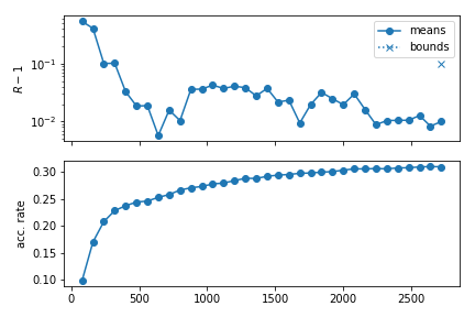
When writing to the hard drive, the MCMC sampler produces an additional [output_prefix].progress file containing the acceptance rate and the Gelman \(R-1\) diagnostics (for means and confidence level contours) per checkpoint, so that the user can monitor the convergence of the chain. In interactive mode (when running inside a Python script of in the Jupyter notebook), an equivalent progress table in a pandas.DataFrame is returned among the products.
The mcmc module provides a plotting tool to produce a graphical representation of convergence, see plot_progress(). An example plot can be seen below:
from cobaya.samplers.mcmc import plot_progress
# Assuming chain saved at `chains/gaussian`
plot_progress("chains/gaussian", fig_args={"figsize": (6,4)})
import matplotlib.pyplot as plt
plt.tight_layout()
plt.show()
When writing to the hard drive (i.e. when an [output_prefix].progress file exists), one can produce these plots even if the sampler is still running.
Callback functions
A callback function can be specified through the callback_function option. It must be a function of a single argument, which at runtime is the current instance of the mcmc sampler. You can access its attributes and methods inside your function, including the SampleCollection of chain points and the model (of which prior and likelihood are attributes). For example, the following callback function would print the points added to the chain since the last callback:
def my_callback(sampler):
    print(sampler.collection[sampler.last_point_callback:])
The callback function is called every callback_every points have been added to the chain, or at every checkpoint if that option has not been defined.
Loading chains (single or multiple)
To load the result of an MCMC run saved with prefix e.g. chains/test as a single chain, skipping the first third of each chain, simply do
from cobaya import load_samples

# As Cobaya SampleCollection
full_chain = load_samples("chains/test", skip=0.33, combined=True)

# As GetDist MCSamples
full_chain = load_samples("chains/test", skip=0.33, to_getdist=True)
Interaction with MPI when using MCMC inside your own script
When integrating Cobaya in your pipeline inside a Python script (as opposed to calling it with cobaya-run), you need to be careful when using MPI: exceptions will not me caught properly unless some wrapping is used:
from mpi4py import MPI

comm = MPI.COMM_WORLD
rank = comm.Get_rank()

from cobaya import run
from cobaya.log import LoggedError

success = False
try:
    upd_info, mcmc = run(info)
    success = True
except LoggedError as err:
    pass

# Did it work? (e.g. did not get stuck)
success = all(comm.allgather(success))

if not success and rank == 0:
    print("Sampling failed!")
In this case, if one of the chains fails, the rest will learn about it and raise an exception too as soon as they arrive at the next checkpoint (in order for them to be able to learn about the failing process earlier, we would need to have used much more aggressive MPI polling in Cobaya, that would have introduced a lot of communication overhead).
As sampler products, every MPI process receives its own chain via the products() method. To gather all of them in the root process and combine them, skipping the first third of each, do:
# Run from all MPI processes at once.
# Returns the combined chain for all of them.

# As cobaya.collections.SampleCollection
full_chain = mcmc.samples(combined=True, skip_samples=0.33)

# As GetDist MCSamples
full_chain = mcmc.samples(combined=True, skip_samples=0.33, to_getdist=True)
Note
For Cobaya v3.2.2 and older, or if one prefers to do it by hand:
all_chains = comm.gather(mcmc.products()["sample"], root=0)

# Pass all of them to GetDist in rank = 0

if rank == 0:
    from getdist.mcsamples import MCSamplesFromCobaya
    gd_sample = MCSamplesFromCobaya(upd_info, all_chains)

# Manually concatenate them in rank = 0 for some custom manipulation,
# skipping 1st 3rd of each chain

copy_and_skip_1st_3rd = lambda chain: chain[int(len(chain) / 3):]
if rank == 0:
    full_chain = copy_and_skip_1st_3rd(all_chains[0])
    for chain in all_chains[1:]:
        full_chain.append(copy_and_skip_1st_3rd(chain))
    # The combined chain is now `full_chain`
Options and defaults
Simply copy this block in your input yaml file and modify whatever options you want (you can delete the rest).
# Default arguments for the Markov Chain Monte Carlo sampler
# ('Xd' means 'X steps per dimension', or full parameter cycle
#  when adjusting for oversampling / dragging)

# Number of discarded burn-in samples per dimension (d notation means times dimension)
burn_in: 0
# Error criterion: max attempts (= weight-1) before deciding that the chain
# is stuck and failing. Set to `.inf` to ignore these kind of errors.
max_tries: 40d
# File (including path) or matrix defining a covariance matrix for the proposal:
# - null (default): will be generated from params info (prior and proposal)
# - matrix: remember to set `covmat_params` to the parameters in the matrix
# - "auto" (cosmology runs only): will be looked up in a library
covmat:
covmat_params:
# Overall scale of the proposal pdf (increase for longer steps)
proposal_scale: 2.4
# Update output file(s) and print some info
# every X seconds (if ends in 's') or X accepted samples (if just a number)
output_every: 60s
# Number of distinct accepted points between proposal learn & convergence checks
learn_every: 40d
# Posterior temperature: >1 for more exploratory chains
temperature: 1
# Proposal covariance matrix learning
# -----------------------------------
learn_proposal: True
# Don't learn if convergence is worse than...
learn_proposal_Rminus1_max: 2.
# (even earlier if a param is not in the given covariance matrix)
learn_proposal_Rminus1_max_early: 30.
# ... or if it is better than... (no need to learn, already good!)
learn_proposal_Rminus1_min: 0.
# Convergence and stopping
# ------------------------
# Maximum number of accepted steps
max_samples: .inf
# Gelman-Rubin R-1 on means
Rminus1_stop: 0.01
# Gelman-Rubin R-1 on std deviations
Rminus1_cl_stop: 0.2
Rminus1_cl_level: 0.95
# When no MPI used, number of fractions of the chain to compare
Rminus1_single_split: 4
# Exploiting speed hierarchy
# --------------------------
# Whether to measure actual speeds for your machine/threading at starting rather
# than using stored values
measure_speeds: True
# Amount of oversampling of each parameter block, relative to their speeds
# Value from 0 (no oversampling) to 1 (spend the same amount of time in all blocks)
# Can be larger than 1 if extra oversampling of fast blocks required.
oversample_power: 0.4
# Thin chain by total oversampling factor (ignored if drag: True)
# NB: disabling it with a non-zero `oversample_power` may produce a VERY LARGE chains
oversample_thin: True
# Dragging: simulates jumps on slow params when varying fast ones
drag: False
# Manual blocking
# ---------------
# Specify parameter blocks and their correspondent oversampling factors
# (may be useful e.g. if your likelihood has some internal caching).
# If used in combination with dragging, assign 1 to all slow parameters,
# and a common oversampling factor to the fast ones.
blocking:
#  - [oversampling_factor_1, [param_1, param_2, ...]]
#  - etc.
# Callback function
# -----------------
callback_function:
callback_every:  # default: every checkpoint
# Seeding runs
# ------------
# NB: in parallel runs, only works until to the first proposer covmat update.
seed:  # integer between 0 and 2**32 - 1
# DEPRECATED
# ----------------
check_every:  # now it is learn_every
oversample: # now controlled by oversample_power > 0
drag_limits:  # use oversample_power instead
Module documentation
- Synopsis:
Blocked fast-slow Metropolis sampler (Lewis 1304.4473)
- Author:
Antony Lewis (for the CosmoMC sampler, wrapped for cobaya by Jesus Torrado)
MCMC sampler class
- class samplers.mcmc.MCMC(info_sampler, model, output=None, packages_path=None, name=None)
Adaptive, speed-hierarchy-aware MCMC sampler (adapted from CosmoMC) cite{Lewis:2002ah,Lewis:2013hha}.
- set_instance_defaults()
Ensure that checkpoint attributes are initialized correctly.
- initialize()
Initializes the sampler: creates the proposal distribution and draws the initial sample.
- property i_last_slow_block
Block-index of the last block considered slow, if binary fast/slow split.
- property slow_blocks
Parameter blocks which are considered slow, in binary fast/slow splits.
- property slow_params
Parameters which are considered slow, in binary fast/slow splits.
- property n_slow
Number of parameters which are considered slow, in binary fast/slow splits.
- property fast_blocks
Parameter blocks which are considered fast, in binary fast/slow splits.
- property fast_params
Parameters which are considered fast, in binary fast/slow splits.
- property n_fast
Number of parameters which are considered fast, in binary fast/slow splits.
- get_acceptance_rate(first=0, last=None)
Computes the current acceptance rate, optionally only for
[first:last]subchain.- Return type:
floating
- set_proposer_blocking()
Sets up the blocked proposer.
- set_proposer_initial_covmat(load=False)
Creates/loads an initial covariance matrix and sets it in the Proposer.
- run()
Runs the sampler.
- n(burn_in=False)
Returns the total number of accepted steps taken, including or not burn-in steps depending on the value of the burn_in keyword.
- get_new_sample_metropolis()
Draws a new trial point from the proposal pdf and checks whether it is accepted: if it is accepted, it saves the old one into the collection and sets the new one as the current state; if it is rejected increases the weight of the current state by 1.
- Return type:
Truefor an accepted step,Falsefor a rejected one.
- get_new_sample_dragging()
Draws a new trial point in the slow subspace, and gets the corresponding trial in the fast subspace by “dragging” the fast parameters. Finally, checks the acceptance of the total step using the “dragging” pdf: if it is accepted, it saves the old one into the collection and sets the new one as the current state; if it is rejected increases the weight of the current state by 1.
- Return type:
Truefor an accepted step,Falsefor a rejected one.
- metropolis_accept(logp_trial, logp_current)
Symmetric-proposal Metropolis-Hastings test.
- Return type:
TrueorFalse.
- process_accept_or_reject(accept_state, trial, trial_results)
Processes the acceptance/rejection of the new point.
- check_ready()
Checks if the chain(s) is(/are) ready to check convergence and, if requested, learn a new covariance matrix for the proposal distribution.
- check_convergence_and_learn_proposal()
Checks the convergence of the sampling process, and, if requested, learns a new covariance matrix for the proposal distribution from the covariance of the last samples.
This method assumes that it will only be called when a checkpoint is reached for all chains.
- do_output(date_time)
Writes/updates the output products of the chain.
- write_checkpoint()
Writes/updates the checkpoint file.
- converge_info_changed(old_info, new_info)
Whether convergence parameters have changed between two inputs.
- samples(combined=False, skip_samples=0, to_getdist=False)
Returns the sample of accepted steps.
- Parameters:
combined (bool, default: False) – If
Trueand running more than one MPI process, returns for all processes a single sample collection including all parallel chains concatenated, instead of the chain of the current process only. For this to work, this method needs to be called from all MPI processes simultaneously.skip_samples (int or float, default: 0) – Skips some amount of initial samples (if
int), or an initial fraction of them (iffloat < 1). If concatenating (combined=True), skipping is applied before concatenation. Forces the return of a copy.to_getdist (bool, default: False) – If
True, returns a singlegetdist.MCSamplesinstance, containing all samples, for all MPI processes (combinedis ignored).
- Returns:
The sample of accepted steps.
- Return type:
SampleCollection, getdist.MCSamples
- products(combined=False, skip_samples=0, to_getdist=False)
Returns the products of the sampling process.
- Parameters:
combined (bool, default: False) – If
Trueand running more than one MPI process, thesamplekey of the returned dictionary contains a sample including all parallel chains concatenated, instead of the chain of the current process only. For this to work, this method needs to be called from all MPI processes simultaneously.skip_samples (int or float, default: 0) – Skips some amount of initial samples (if
int), or an initial fraction of them (iffloat < 1). If concatenating (combined=True), skipping is applied previously to concatenation. Forces the return of a copy.to_getdist (bool, default: False) – If
True, thesamplekey of the returned dictionary contains a singlegetdist.MCSamplesinstance including all samples (combinedis ignored).
- Returns:
A dictionary containing the sample of accepted steps under
sample(ascobaya.collection.SampleCollectionby default, or asgetdist.MCSamplesifto_getdist=True), and a progress report table under"progress".- Return type:
dict
- classmethod output_files_regexps(output, info=None, minimal=False)
Returns regexps for the output files created by this sampler.
- classmethod get_version()
Returns the version string of this samples (since it is built-in, that of Cobaya).
Progress monitoring
- samplers.mcmc.plot_progress(progress, ax=None, index=None, figure_kwargs=mappingproxy({}), legend_kwargs=mappingproxy({}))
Plots progress of one or more MCMC runs: evolution of R-1 (for means and c.l. intervals) and acceptance rate.
Takes a
progressinstance (actually apandas.DataFrame, returned as part of the samplerproducts), a chainoutputprefix, or a list of those for plotting progress of several chains at once.You can use
figure_kwargsandlegend_kwargsto pass arguments tomatplotlib.pyplot.figureandmatplotlib.pyplot.legendrespectively.Returns a subplots axes array. Display with
matplotlib.pyplot.show().
Proposal
- Synopsis:
proposal distributions
- Author:
Antony Lewis and Jesus Torrado
Using the covariance matrix to give the proposal directions typically significantly increases the acceptance rate and gives faster movement around parameter space.
We generate a random basis in the eigenvectors, then cycle through them proposing changes to each, then generate a new random basis. The distance proposal in the random direction is given by a two-D Gaussian radial function mixed with an exponential, which is quite robust to wrong width estimates
See https://arxiv.org/abs/1304.4473
- class samplers.mcmc.proposal.CyclicIndexRandomizer(n, random_state)
- next()
Get the next random index, or alternate for two or less.
- Returns:
index
- class samplers.mcmc.proposal.RandDirectionProposer(n, random_state)
- propose_vec(scale=1)
Propose a random n-dimension vector for n>1
- Parameters:
scale (
float) – units for the distance- Returns:
array with vector
- propose_r()
Radial proposal. By default a mixture of an exponential and 2D Gaussian radial proposal (to make wider tails and more mass near zero, so more robust to scale misestimation)
- Returns:
random distance (unit scale)
- class samplers.mcmc.proposal.BlockedProposer(parameter_blocks, random_state, oversampling_factors=None, i_last_slow_block=None, proposal_scale=2.4)
- set_covariance(propose_matrix)
Take covariance of sampled parameters (propose_matrix), and construct orthonormal parameters where orthonormal parameters are grouped in blocks by speed, so changes in the slowest block changes slow and fast parameters, but changes in the fastest block only changes fast parameters
- Parameters:
propose_matrix – covariance matrix for the sampled parameters.