Creating your own cosmological likelihood
Creating your own cosmological likelihood with cobaya is super simple. You can either define a likelihood class (see Creating your own cosmological likelihood class), or simply create a likelihood function:
Define your likelihood as a function that takes some parameters (experimental errors, foregrounds, etc, but not theory parameters) and returns a
log-likelihood.Take note of the observables and other cosmological quantities that you will need to request from the theory code (see
must_provide()). [If you cannot find the observable that you need, do let us know!]When declaring the function as a likelihood in cobaya’s input, add a field
requiresand assign to it all the cosmological requirements as a dictionary (e.g.{'Cl': {'tt': 2500}}).Add to your likelihood function definition a keyword argument
_self=None. At run-time, you can callget_[...]methods of_self.providerto get the quantities that you requested evaluated at the current parameters values, e.g_self.provider.get_Cl()in the example below.If you wish to define derived paramters, do it as for general external likelihoods (example here): add an
output_paramsfield to the likelihood info listing your derived parameters, and have your function return a tuple(log-likelihood, {derived parameters dictionary}).
Example: your own CMB experiment!
To illustrate how to create a cosmological likelihood in cobaya, we apply the procedure above to a fictitious WMAP-era full-sky CMB TT experiment.
First of all, we will need to simulate the fictitious power spectrum of the fictitious sky that we would measure with our fictitious experiment, once we have accounted for noise and beam corrections. To do that, we choose a set of true cosmological parameters in the sky, and then use a model to compute the corresponding power spectrum, up to some reasonable \(\ell_\mathrm{max}\) (see Using the model wrapper).
fiducial_params = {
    'ombh2': 0.022, 'omch2': 0.12, 'H0': 68, 'tau': 0.07,
    'As': 2.2e-9, 'ns': 0.96,
    'mnu': 0.06, 'nnu': 3.046}

l_max = 1000

packages_path = '/path/to/your/packages'

info_fiducial = {
    'params': fiducial_params,
    'likelihood': {'one': None},
    'theory': {'camb': {"extra_args": {"num_massive_neutrinos": 1}}},
    'packages_path': packages_path}

from cobaya.model import get_model
model_fiducial = get_model(info_fiducial)

# Declare our desired theory product
# (there is no cosmological likelihood doing it for us)
model_fiducial.add_requirements({"Cl": {'tt': l_max}})

# Compute and extract the CMB power spectrum
# (In muK^-2, without l(l+1)/(2pi) factor)
# notice the empty dictionary below: all parameters are fixed
model_fiducial.logposterior({})
Cls = model_fiducial.provider.get_Cl(ell_factor=False, units="muK2")

# Our fiducial power spectrum
Cl_est = Cls['tt'][:l_max + 1]
Now, let us define the likelihood. The arguments of the likelihood function will contain the parameters that we want to vary (arguments not mentioned later in an input info will be left to their default, e.g. beam_FWHM=0.25). As mentioned above, include a _self=None keyword from which you will get the requested quantities, and, since we want to define derived parameters, return them as a dictionary:
import numpy as np
import matplotlib.pyplot as plt

_do_plot = False

def my_like(
        # Parameters that we may sample over (or not)
        noise_std_pixel=20,  # muK
        beam_FWHM=0.25,  # deg
        # Keyword through which the cobaya likelihood instance will be passed.
        _self=None):
    # Noise spectrum, beam-corrected
    healpix_Nside=512
    pixel_area_rad = np.pi/(3*healpix_Nside**2)
    weight_per_solid_angle = (noise_std_pixel**2 * pixel_area_rad)**-1
    beam_sigma_rad = beam_FWHM / np.sqrt(8*np.log(2)) * np.pi/180.
    ells = np.arange(l_max+1)
    Nl = np.exp((ells*beam_sigma_rad)**2)/weight_per_solid_angle
    # Cl of the map: data + noise
    Cl_map = Cl_est + Nl
    # Request the Cl from the provider
    Cl_theo = _self.provider.get_Cl(ell_factor=False, units="muK2")['tt'][:l_max+1]
    Cl_map_theo = Cl_theo + Nl
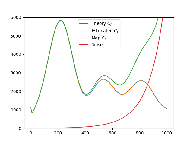
    # Auxiliary plot
    if _do_plot:
        ell_factor = ells*(ells+1)/(2*np.pi)
        plt.figure()
        plt.plot(ells[2:], (Cl_theo*ell_factor)[2:], label=r'Theory $C_\ell$')
        plt.plot(ells[2:], (Cl_est*ell_factor)[2:], label=r'Estimated $C_\ell$', ls="--")
        plt.plot(ells[2:], (Cl_map*ell_factor)[2:], label=r'Map $C_\ell$')
        plt.plot(ells[2:], (Nl*ell_factor)[2:], label='Noise')
        plt.legend()
        plt.ylim([0, 6000])
        plt.savefig(_plot_name)
        plt.close()
    # ----------------
    # Compute the log-likelihood
    V = Cl_map[2:]/Cl_map_theo[2:]
    logp = np.sum((2*ells[2:]+1)*(-V/2 +1/2.*np.log(V)))
    # Set our derived parameter
    derived = {'Map_Cl_at_500': Cl_map[500]}
    return logp, derived
Finally, let’s prepare its definition, including requirements (the CMB TT power spectrum) and listing available derived parameters, and use it to do some plots.
Since our imaginary experiment isn’t very powerful, we will refrain from trying to estimate the full \(\Lambda\) CDM parameter set. We may focus instead e.g. on the primordial power spectrum parameters \(A_s\) and \(n_s\) as sampled parameters, assume that we magically have accurate values for the rest of the cosmological parameters, and marginalise over some uncertainty on the noise standard deviation
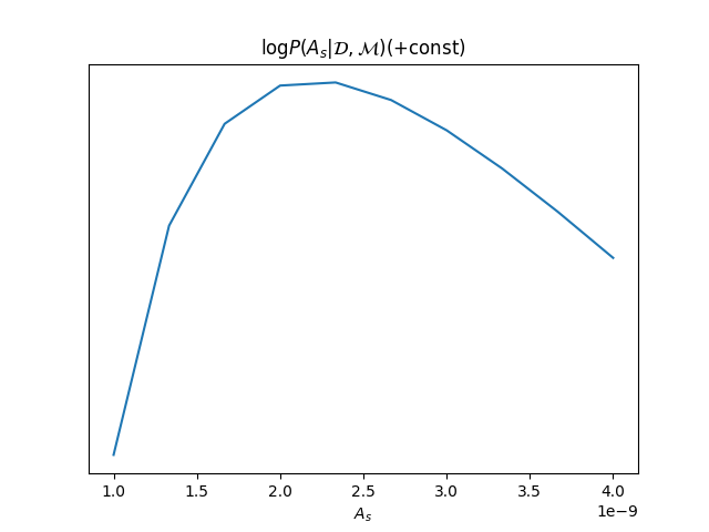
We will define a model, use our likelihood’s plotter, and also plot a slice of the log likelihood along different \(A_s\) values:
info = {
    'params': {
        # Fixed
        'ombh2': 0.022, 'omch2': 0.12, 'H0': 68, 'tau': 0.07,
        'mnu': 0.06, 'nnu': 3.046,
        # Sampled
        'As': {'prior': {'min': 1e-9, 'max': 4e-9}, 'latex': 'A_s'},
        'ns': {'prior': {'min': 0.9, 'max': 1.1}, 'latex': 'n_s'},
        'noise_std_pixel': {
            'prior': {'dist': 'norm', 'loc': 20, 'scale': 5},
            'latex': r'\sigma_\mathrm{pix}'},
        # Derived
        'Map_Cl_at_500': {'latex': r'C_{500,\,\mathrm{map}}'}},
    'likelihood': {'my_cl_like': {
        "external": my_like,
        # Declare required quantities!
        "requires": {'Cl': {'tt': l_max}},
        # Declare derived parameters!
        "output_params": ['Map_Cl_at_500']}},
    'theory': {'camb': {'stop_at_error': True}},
    'packages_path': packages_path}

from cobaya.model import get_model
model = get_model(info)

# Eval likelihood once with fid values and plot
_do_plot = True
_plot_name = "fiducial.png"
fiducial_params_w_noise = fiducial_params.copy()
fiducial_params_w_noise['noise_std_pixel'] = 20
model.logposterior(fiducial_params_w_noise)
_do_plot = False

# Plot of (prpto) probability density
As = np.linspace(1e-9, 4e-9, 10)
loglikes = [model.loglike({'As': A, 'ns': 0.96, 'noise_std_pixel': 20})[0] for A in As]
plt.figure()
plt.plot(As, loglikes)
plt.gca().get_yaxis().set_visible(False)
plt.title(r"$\log P(A_s|\mathcal{D},\mathcal{M}) (+ \mathrm{const})$")
plt.xlabel(r"$A_s$")
plt.savefig("log_like.png")
plt.close()


Note
Troubleshooting:
If you are not getting the expected value for the likelihood, here are a couple of things that you can try:
Set
debug: Truein the input, which will cause cobaya to print much more information, e.g. the parameter values are passed to the prior, the theory code and the likelihood.If the likelihood evaluates to
-inf(but the prior is finite) it probably means that either the theory code or the likelihood are failing; to display the error information of the theory code, add to it thestop_at_error: Trueoption, as shown in the example input above, and the same for the likelihood, if it is likely to throw errors.
Now we can sample from this model’s posterior as explained in Interacting with a sampler.
Alternatively, specially if you are planning to share your likelihood, you can put its definition (including the fiducial spectrum, maybe saved as a table separately) in a separate file, say my_like_file.py. In this case, to use it, use import_module([your_file_without_extension]).your_function, here
# Contents of some .yaml input file
likelihood:
    some_name:
        external: import_module('my_like_file').my_like
        # Declare required quantities!
        requires: {Cl: {tt: 1000}}
        # Declare derived parameters!
        output_params: [Map_Cl_at_500]